None
Note
This tutorial was generated from an IPython notebook that can be downloaded here.
Usage example
import pyspatialstats.focal as fs
import rasterio as rio
import matplotlib.pyplot as plt
import numpy as np
import os
os.chdir('../../../')
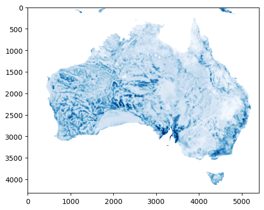
Loading raster (containing water table depth (Fan et al., 2017)).
with rio.open('data/wtd.tif') as f:
    a = f.read(1).astype(np.float64)
    a[a == -999.9] = np.nan
Inspecting the data
plt.imshow(a, cmap='Blues', vmax=100)
plt.title('Water table depth')
plt.colorbar()
<matplotlib.colorbar.Colorbar at 0x153e75010>

Focal statistics
Calculation of the focal mean:
plt.imshow(fs.focal_mean(a, window=15).mean, vmax=100, cmap='Blues')
<matplotlib.image.AxesImage at 0x153fee850>

This looks quite similar to the input raster, but with smoothing applied. Let’s try a higher window, which should increase the smoothing
plt.imshow(fs.focal_mean(a, window=25).mean, vmax=100, cmap='Blues')
<matplotlib.image.AxesImage at 0x15407a210>
This same functionality can be used to reduce the shape of the raster based on this window.
x = fs.focal_mean(a, window=108, reduce=True).mean
plt.imshow(x, vmax=100, cmap='Blues')
<matplotlib.image.AxesImage at 0x1541056d0>
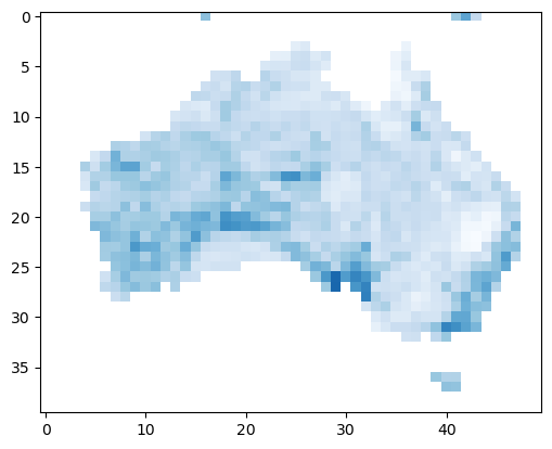
The shape of this new raster is exactly 108 times smaller than the input raster. Note that for this to work both x and y-axes need to be divisible by the window size.